You built the perfect formula. You checked every range twice. You hit Enter — and Google Sheets slaps you with a cold, unhelpful #N/A.
If you've ever tried to look something up by two conditions at once — a price that depends on both the product and the region, a score that depends on the student and the subject — you've probably lived this exact moment. The formula looks right. It even works if you paste it into Excel. So why does Google Sheets refuse to play along?
Take a breath. You're not doing anything wrong. Google Sheets just treats one specific thing differently from Excel, and once you know the one-word fix, multi-criteria XLOOKUP becomes something you'll reach for every week. Let's build it up properly — from the ground.
First, a quick refresher on how XLOOKUP works
Before we combine conditions, let's make sure the foundation is solid, because the fix only makes sense once you see what XLOOKUP is really doing.
A basic XLOOKUP has three parts:
=XLOOKUP(what_to_find, where_to_look, what_to_return)
So if you had a list of products in column A and prices in column C, =XLOOKUP("Banana", A2:A6, C2:C6) walks down column A, finds the row that says "Banana," and hands back the price sitting next to it. Simple, clean, and much friendlier than the old VLOOKUP.
The catch: XLOOKUP is built to match one thing. Give it a single product and it's happy. Ask it to match a product and a region at the same time, and there's no obvious slot for that second condition. That's where people get stuck.
The real-world problem: one criterion isn't enough
Here's the kind of table that breaks a plain lookup:
| Product | Region | Price |
|---|---|---|
| Apple | North | 120 |
| Apple | South | 95 |
| Banana | North | 60 |
| Banana | South | 75 |
| Cherry | North | 200 |
Notice that Apple appears twice — once for North, once for South. If you just do =XLOOKUP("Apple", A2:A6, C2:C6), Google Sheets returns 120, because it stops at the first Apple it finds. But you didn't want any Apple — you wanted Apple in the South, which is 95.
So you need to match two columns at once. Let's put the two things we're searching for in their own cells — F1 holds Apple, F2 holds South — and go find that 95.
The formula everyone tries first (and why it feels so right)
Search around and you'll land on this clever trick:
=XLOOKUP(1,(A2:A6=F1)*(B2:B6=F2),C2:C6)
The logic is genuinely beautiful. (A2:A6=F1) gives you a little list of TRUE/FALSE — TRUE on every row where the product is Apple. (B2:B6=F2) does the same for South. Multiply those two lists together and TRUE×TRUE becomes 1, while anything else becomes 0. So you end up with a single 1 sitting on the exact row where both conditions are met — and you just tell XLOOKUP to go find that 1.
Paste it into Excel and it works instantly. Paste it into Google Sheets and… #N/A. Infuriating, because the thinking is correct.
…and here's why Google Sheets says #N/A
The difference is subtle but important. When you multiply those two TRUE/FALSE lists inside the formula, you're asking Google Sheets to do array math — to calculate a whole column of values in one go.
Excel does that automatically inside XLOOKUP. Google Sheets does not. Left on its own, Sheets doesn't expand (A2:A6=F1)*(B2:B6=F2) into a real list — so XLOOKUP never actually sees your column of 1s and 0s, finds nothing to match against 1, and throws #N/A. It's not a mistake in your logic; it's a difference in how the two apps evaluate arrays.
The one-word fix: ARRAYFORMULA
You just have to tell Google Sheets, explicitly, "hey — treat this as an array." That word is ARRAYFORMULA. Wrap it around the multiplied condition:
=XLOOKUP(1,ARRAYFORMULA((A2:A6=F1)*(B2:B6=F2)),C2:C6)
Hit Enter, and there it is: 95 — the price of Apple in the South.
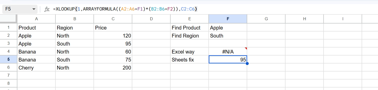
That one word is the entire difference between #N/A and a working formula. Everything else you already had was right.
How it actually works (so you can adapt it to anything)
Let's slow down on the mechanics, because once this clicks you can reuse it for any lookup, with any number of conditions.
(A2:A6=F1)→{TRUE; TRUE; FALSE; FALSE; FALSE}— which rows are Apple(B2:B6=F2)→{FALSE; TRUE; FALSE; TRUE; FALSE}— which rows are South- multiply them →
{0; 1; 0; 0; 0}— a 1 appears only on the row where both are true ARRAYFORMULA(...)forces Sheets to actually build that list of 1s and 0sXLOOKUP(1, that_list, C2:C6)finds the single1and returns the price on that row → 95
The pattern is: build a column that's 1 only on the matching row, then look up the 1. Need a third condition? Just multiply in another one: ... * (D2:D6=F3). The idea scales as far as you need.
Two other ways to do the same thing
XLOOKUP is great, but it's not the only tool. These both return 95 in Google Sheets too, and they're worth knowing:
=FILTER(C2:C6, A2:A6=F1, B2:B6=F2)
=INDEX(C2:C6, MATCH(1, (A2:A6=F1)*(B2:B6=F2), 0))
FILTER is often the cleanest for multiple conditions — you just list them one after another, no ARRAYFORMULA needed. Reach for it when you might have more than one matching row and want them all. INDEX/MATCH is the classic that's been solving this since long before XLOOKUP existed; handy if you're working in an older sheet or sharing with Excel users. Use whichever fits — they all get you to the same answer.
Common mistakes that still throw #N/A
If you're still seeing #N/A after adding ARRAYFORMULA, check these:
- A stray space. "South " with a trailing space won't match "South". Clean your data with
TRIM(). - Text vs. number. Looking up
95(a number) against prices stored as text ("95") fails silently. Keep types consistent. - Mismatched ranges.
A2:A6andB2:B7are different lengths — every range in the formula must cover the same rows. - A real no-match. Sometimes
#N/Ais honest: that combination genuinely isn't in the table. Add a friendly fallback with the fourth argument:=XLOOKUP(1, ARRAYFORMULA(...), C2:C6, "Not found").
The pattern to remember
=XLOOKUP(1, ARRAYFORMULA((condition1) * (condition2)), result_range)
Wrap your multiplied conditions in ARRAYFORMULA, look up the 1, and multi-criteria XLOOKUP works every single time in Google Sheets. Bookmark that template — you'll use it more than you think.
FAQ
Why does my XLOOKUP return #N/A in Google Sheets but works in Excel?
Because Google Sheets doesn't automatically evaluate the multiplied (range=value)*(range=value) condition as an array the way Excel does. Wrap that condition in ARRAYFORMULA and it works: =XLOOKUP(1, ARRAYFORMULA((A2:A6=F1)*(B2:B6=F2)), C2:C6).
Can XLOOKUP handle three or more criteria?
Yes. Just multiply in each extra condition inside the ARRAYFORMULA: ARRAYFORMULA((A2:A6=F1)*(B2:B6=F2)*(C2:C6=F3)). The row where all conditions are true becomes 1, and XLOOKUP finds it.
Is FILTER better than XLOOKUP for multiple criteria?
FILTER is often simpler — you list conditions one after another with no ARRAYFORMULA — and it's the better choice when more than one row can match and you want every result. Use XLOOKUP when you expect a single answer and like its clean syntax.
How do I stop the #N/A and show a message instead?
Add a fallback as XLOOKUP's fourth argument: =XLOOKUP(1, ARRAYFORMULA((A2:A6=F1)*(B2:B6=F2)), C2:C6, "Not found"). Now a missing combination shows "Not found" instead of an error.
That's the whole trick. It's not that your logic was wrong — Google Sheets just needed one extra word to evaluate it. Add ARRAYFORMULA, and multi-criteria XLOOKUP goes from "why won't this work?!" to a formula you'll trust every time.
Want more short, practical spreadsheet and AI-tool guides that actually solve the problem? New tutorials drop every week — grab them below.


